
In Part I of our demand forecasting series, we discussed the fundamental concepts of demand, the law of demand, price elasticity, and how these core ideas shape consumer behavior. Now, we shift our focus to how demand evolves over time, and more importantly, how we can predict future demand using time series models.
Time series forecasting is one of the most powerful tools in a business analyst’s arsenal. In this article, we will explore different time series models, delve into the mathematics behind them, implement a working ARIMA model in Python, and validate our forecast using statistical tools. Let’s begin.
Understanding Time Series in Demand Modeling
A time series is a sequence of observations recorded over time. In demand modeling, this could include daily product sales, monthly revenue, or weekly website visits. Time series data typically shows three components:
- Trend: A long-term increase or decrease in the data.
- Seasonality: Repeating short-term cycles (e.g., increased demand during holidays).
- Noise/Residual: Random variation that cannot be explained by trend or seasonality.
Forecasting demand with time series data allows businesses to anticipate future needs and optimize operations accordingly.
1. ARIMA (AutoRegressive Integrated Moving Average)
ARIMA is one of the most widely used models in time series forecasting. It is ideal for univariate data (i.e., one time-dependent variable like past demand).
Mathematical Formulation:
An ARIMA(p,d,q) model is composed of:
- AR(p): Autoregressive term. Models the variable as a linear combination of past values.
- I(d): Integrated term. The number of times the data needs to be differenced to become stationary.
- MA(q): Moving average term. Models the variable as a linear combination of past forecast errors.
The general ARIMA model equation:
$ Y_t=c+ϕ_1Y_{t−1}+…+ϕ_pY_{t−p}+θ_1ε_{t−1}+…+θ_qε_{t−q}+ε_t $
Where:
- $ϕ$ are the autoregressive parameters
- $θ$ are the moving average parameters
- $ε_t$ is white noise
Stationarity and Differencing
Time series must be stationary (constant mean and variance over time) for ARIMA to work. This is often achieved by differencing the series:
$ Y’_t = Y_t – Y_{t-1} $
We verify stationarity using the Augmented Dickey-Fuller (ADF) test.
ADF Test (Python Example)
from statsmodels.tsa.stattools import adfuller
result = adfuller(demand_data)
print('ADF Statistic:', result[0])
print('p-value:', result[1])
If p-value < 0.05, we reject the null hypothesis and the series is stationary.
Python Implementation: ARIMA Model
import pandas as pd
from statsmodels.tsa.arima.model import ARIMA
from matplotlib import pyplot as plt

# Load dataset
data = pd.read_csv('demand.csv', index_col='Date', parse_dates=True)
series = data['Quantity']

# Fit ARIMA model
model = ARIMA(series, order=(1,1,1))
model_fit = model.fit()
print(model_fit.summary())

# Plot forecast
forecast = model_fit.forecast(steps=12)
plt.plot(series)
plt.plot(forecast, color='red')
plt.title('ARIMA Forecast')
plt.show()
2. OLS (Ordinary Least Squares) Regression
OLS models the relationship between a dependent variable and one or more independent variables.
Equation:
$ Q_d=β_0+β_1P+β_2X_2+…+β_nX_n+ε $
Where:
- $ Q_d $ is quantity demanded
- P is price
- $ X_n $ are other variables (e.g., ads, discounts)
- $ ε $ is the error term
OLS is useful for understanding how specific variables (like price or promotions) influence demand, but it assumes a static relationship and may not handle temporal dynamics well.
3. VAR (Vector AutoRegression)
VAR is used when multiple time series influence each other. For example, product demand might depend on ad spend, consumer income, and other product sales.
Each variable in VAR is modeled as a function of lags of itself and lags of all other variables.
VAR Equation for 2 Variables:
$ Y_t=A_1Y_{t−1}+A_2Y_{t−2}+…+A_pY_{t−p}+ε_t $
Where $ Y_t $ is a vector of variables like Demand.
Interpreting ACF and PACF Plots
- ACF (Autocorrelation Function): Measures correlation between the series and its lagged values.
- PACF (Partial ACF): Measures the correlation after removing the effect of intermediate lags.
These plots help determine the appropriate values of p and q in ARIMA.
Python Example:
from statsmodels.graphics.tsaplots import plot_acf, plot_pacf
plot_acf(demand_data)
plot_pacf(demand_data)
Forecast Accuracy: MAPE and RMSE
- MAPE: Mean Absolute Percentage Error
$ MAPE=\frac{1}{n}∑∣\frac{A_t−F_t}{A_t}∣×100 $
- RMSE: Root Mean Squared Error
$ RMSE=\sqrt{ \frac{1}{n}∑(A_t−F_t)^2} $
These metrics help evaluate the accuracy of your forecast by comparing predicted values to actual observations. Ideally, you want metrics like Mean Absolute Error (MAE) and Root Mean Square Error (RMSE) to be as low as possible, indicating smaller prediction errors. For Mean Absolute Percentage Error (MAPE), values below 10% are considered highly accurate, 10–20% good, and above 50% poor, depending on the industry context.
from sklearn.metrics import mean_absolute_percentage_error, mean_squared_error

mape = mean_absolute_percentage_error(actual, predicted)
rmse = mean_squared_error(actual, predicted, squared=False)
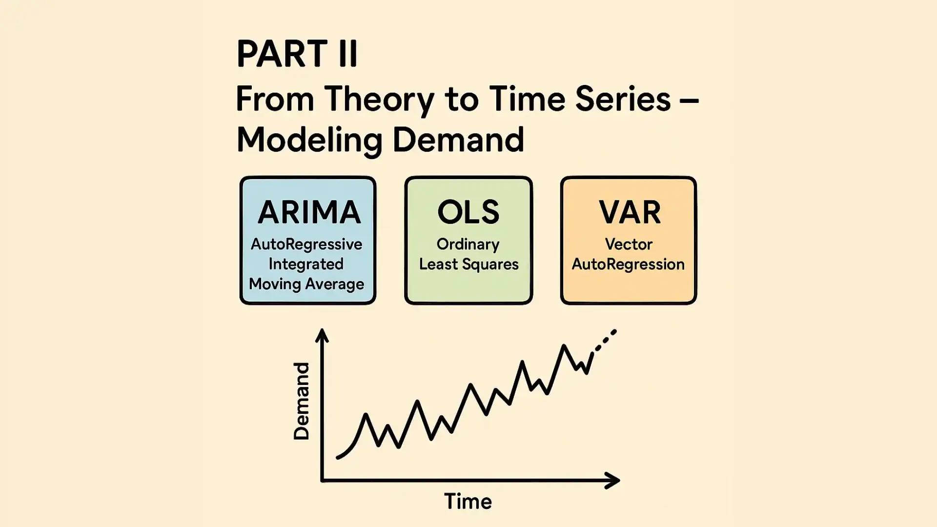
Conclusion
Forecasting demand using time series models like ARIMA, OLS, and VAR enables businesses to stay proactive rather than reactive. By blending economic theory with data science tools, you can move from abstract models to actionable insights that fuel smarter decisions.
In the next part, we’ll look at how real-world e-commerce companies implement these models using cloud-based infrastructure and automation workflows.
Stay tuned.